Simulations to create a distribution of Y-DNA branch sizes of the Ashkenazi Jews
The data
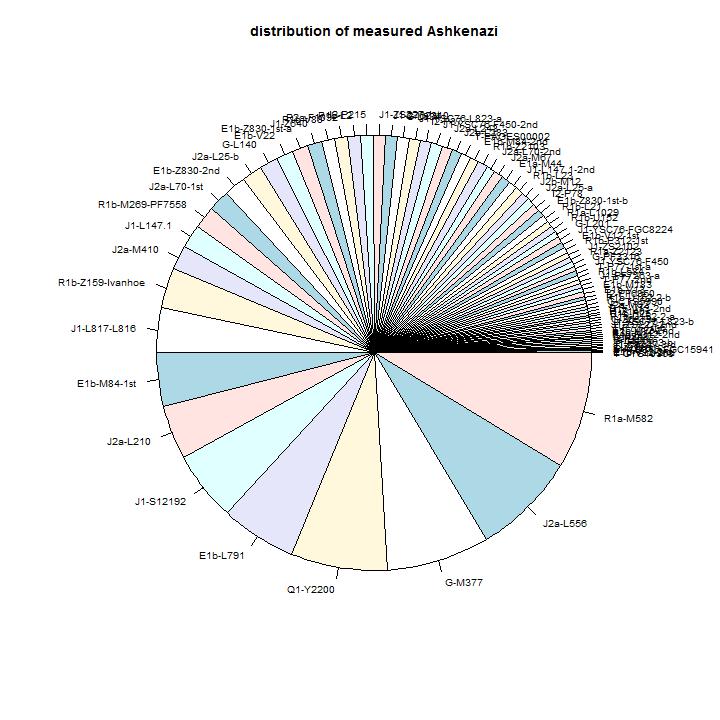
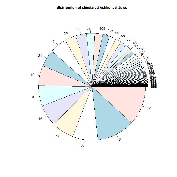
The distribution of sizes of branches, ordered by size.
The models
These models describe the Jews arriving in Polish-Lithuanian Europe.
To find a realistic model, the models should follow a set of observed characteristics. The most important are:
- size of Ashkenazi Jews in recent times
- the number of male line Ashkenazi ancestors
- the variability in the sizes of Ashkenazi Y-DNA branches
- the timescale between Ashkenazi ancestors and present should follow the timescale that was found in Y-DNA time estimates (STR or SNP)
As a measure of the amount of Jews in recent times we used the values of 700.000 in 1620 (see Demographic history of Poland), 1.000.000 in 1770 (see History of Jews in Poland) and 9.000.000 in 1890 (see Historical Jewish population comparisons)
This simulation routines were previously used for the paper on 2000 years genetic variability in Flanders, Brabant and Limburg.
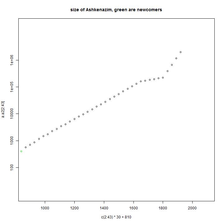
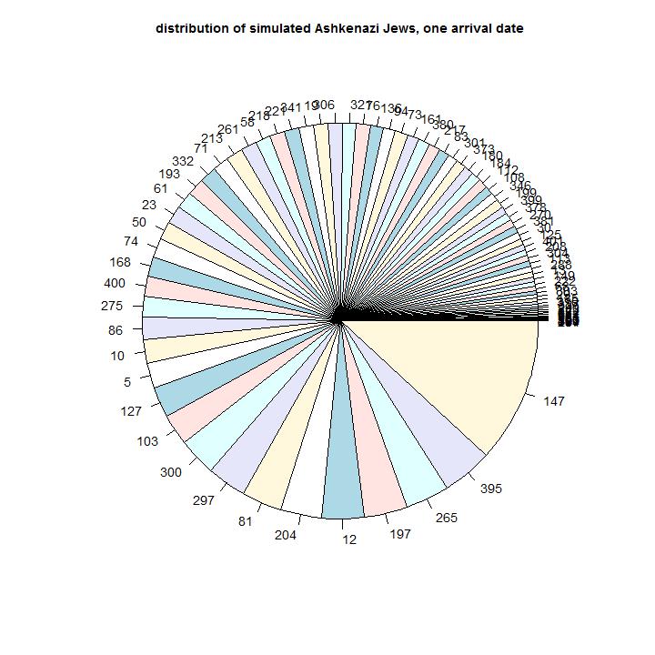
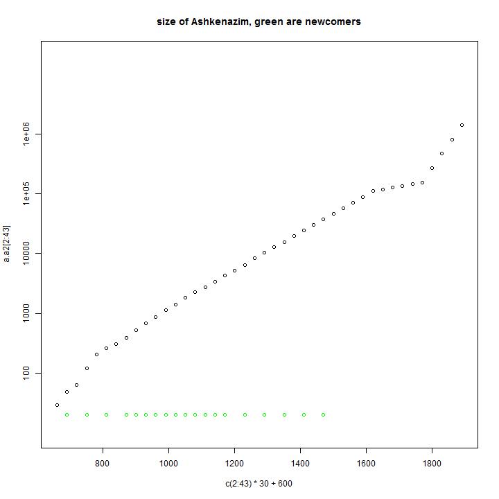
In the first diagram of each model one can see the size of the Ashkenazi as function of time. In this simulation 400 male line ancestors are arriving near the year 800.
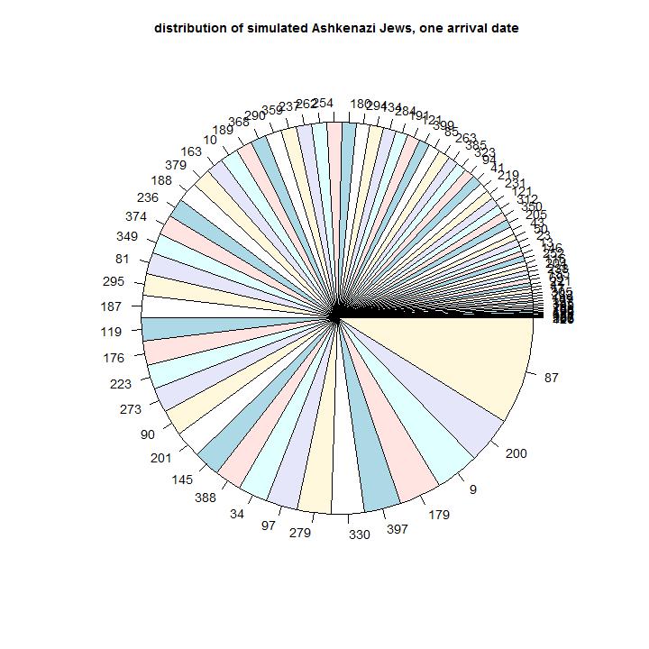
In green the amount of arriving male line ancestors is indicated. In the piechart the sizes of the present simulated haplogroups is indicated. They are ordered in size. The number is the order or the simulated male line ancestor. Most of the male line ancestors will have no male line descendants after many years.
Model 1
Model input: This is the (most simple) model to describe the Jews arriving in Polish-Lithuanian Europe (400 people arriving at the same time and constant grow rate in the period until 1620).
In this model the distribution of the size of the Ashkenazim does not follow the observed distribution.
Simulation results: In this simulation we have descendants of 84 male line ancestors.
Comparison with observations: In the observations we have 8 male line ancestors that have 50% of the Ashkenazi descendants. The diversity of sizes of the different simulated branches is insufficient. This simulation does not describe the distribution sufficiently.
Model 2
Model input: In this model the the growth rate of the people is not stable, but has periods of no growth and stronger growth.
Simulation results: In this simulation we have descendants of 84 male line ancestors.
Comparison with the observations: In this model the distribution is a little bit better than in the previous model, but the fundamental difference between model and data is still present.
Model 3
Model input: In this model we use less ancestors to start with and a larger population growth.
Simulation results: The time of initial arrival of the first Ashkenazi Jews is later. The number of branches is less than the number of Ashkenazi branches and the small branches are lacking.
Comparison with the observations: This model does not have the amount of present branches. It does not describe the diversity of the amount and size of the branches.
Model 4
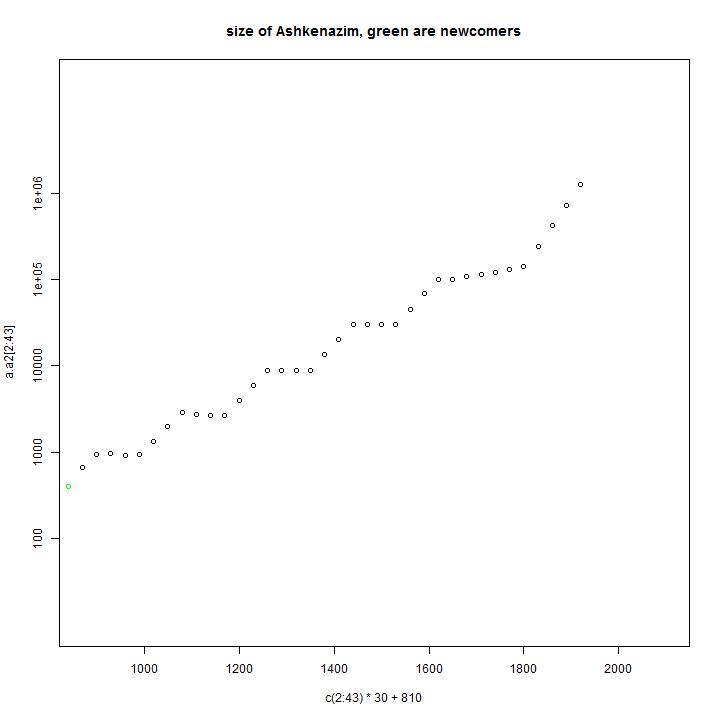
Model input: In this model the 400 people are arriving over a period of time in the area where the population growth is strong. This can be seen by the green dots in the first diagram.
Simulation results: In this simulation we have descendants of 75 male line ancestors.
Comparison with the observations: This model can describe the observed distribution of haplogroups. The numbers describe the arrival times of the groups. As one would expect the present largest groups are the groups that arrived first. The groups that arrived last are the relative small groups.
Model 5
Model input: In this model we assume that we have a difference in status in the community. This might be the case if sons of a elite group in the community have more chance to have descendants.
Simulation results: It is possible to create parameters to realize the distributions. The differences in population growth should be large and the continuation of the differences should last (in the simulated models) about 400 years.
Comparison with the observations: It is possible to make a model to fit the distribution, but the required parameters are unlikely realistic.
General Characteristics of the model
The model has the following characteristics:
- Each grown up male has, on average, the same chance to have male and female descendants. The only parameter that is used is the average population growth of the group. This means that if the population growth of the group is 1.5 in a generation, the group as a total is increased by a factor 1.5.
- The chance that a person has one or more children does not influence the chance to have a child more. This is not the case in a modern society, but is probably a good approximation of historic population growth. For this reason a Poisson distribution is used.
The model has a few parameters:
- length of a generation. In this calculation 30 years is used.
- population growth. This is expressed in this model as the population growth in a period of 30 years. This means that it is the same as the population growth for the length of the chosen generation.
In the model only males that reach the age of becoming a father are calculated in the model; for this reason we the term "potential father" in the model. This means that women and children that do not reach this age are not part of the model. To make the numbers comparable with e.g. population size we should use a ratio of population size to Y-DNA ancestors.
- The ratio of population size to potential fathers was determined for the perdio 1800-1850 in the Netherlands. This ratio was 4.5: the population size was 4.5 the size of the amount of potential fathers. In historic times it is likely that this number was somewhat higher.
The simplest model
In the simplest model we have a population with a stable population growth over a long period of time.
In the document of paper on 2000 years genetic variability in Flanders, Brabant and Limburg it was shown that, as a first approximation, one can use the value of 1.02 for a population growth in the Neolitic period and 1.06 in the period 8000-2000 ybp for the population of R1b in Europe. These two values give the following characteristics of number of parameters:
| typical for period | ? | ? | 8000-2000ybp | short periods or special groups
|
| population growth in 30 years | 1.01 | 1.02 | 1.06 | 1.20
|
| percentage of potential fathers that has a present day descendant | 0.01 | 0.02 | 0.06 | 0.20
|
| mean number of generations of a person that lived once to a shared ancestor of a living person | 60 | 32 | 10 | 3
|
| ratio of population size to Y-DNA found at a moment in time | 450 | 225 | 75 | 25
|
| average number of SNP markers not shared by a living person (using 90years/SNP) | 20 | 10 | 3 | 1
|
| time to double the population size | 2010 years | 1050 years | 360 years | 114 years
|
| time to 10-fold the population size | 6950 years | 3480 years | 1180 years | 380 years
|
Best model
The model that best describes the distribution of branchsizes is Model 4.
It gives an arrival of Ashkenazi Jews over a long period of time, and an effective population
growth that is about 1.25 per generation (using an average generation of 30 years).